Materials¶

Materials are the most painful and error-prone items to transfer from code to code, since each MC code specifies materials in a different way. Instead, we tag groups of volumes with a name and syntax that corresponds to material compositions in a predefined material library.

The group naming syntax for describing materials in Cubit is:

CUBIT> group "mat:<Name of Material>"

If you wish to specify a material that is present in the library with a different density, then

CUBIT> group "mat:<Name of Material>/rho:<density>"

So for example, to specify a Stainless Steel at a density of 12.0 g/cc,

CUBIT> group "mat:Stainless Steel/rho:12.0"

Scoring¶

Each MC code implements tallies, or scores, in very specific ways such that there is sometimes no equivalent to a tally you may be familiar with, code to code. However, there is a Cubit syntax to allow you to request scores on geomemtric elments. The generic form is

CUBIT> group "tally:ParticleName/ScoreType" add vol x

A specific example, scoring the neutron flux in vol 2,

CUBIT> group "tally:Neutron/Flux" add vol 2

or the photon current crossing surface 3,

CUBIT> group "tally:Photon/Current" add surface 3

Using the underlying PyNE libraries, we can write out the appropriate MC code tally specification snippet; this allows the number of codes that DAGMC supports to grow organically with those that PyNE supports. When PyNE cannot fulfill your tally request it will warn you.

Boundary conditions¶

All MC codes have an understanding of boundary conditions, and all at least implement some form of graveyard, black hole or region where particles are “killed”. Some MC codes go further and define reflecting or other boundary conditions. Furthermore, some apply these boundary conditions to entire volumes as opposed to surfaces. Currently we support only reflecting surface definitions, but in the near term we hope to support full volume reflecting boundaries. One can implement reflecting surfaces in UW² by adding surfaces to the following Cubit group defintion

CUBIT> group "boundary:Reflecting"

or if you prefer, Lambert (white reflection)

CUBIT> group "boundary:White"

Particle importances¶

Particle importances are in important aspect of Monte Carlo simulations and are used to help particles to penetrate to “important” regions of the geometry. There are several automatic methods to generate mesh based importances or weights, but if your importances are tried to the geometry, then they can be tagged onto the geometry.

The UW² workflow has a code agnostic way of defining importances.

CUBIT> group "importance:Neutron/1.0"

This is translated to the code specific version at runtime. Note: Fluka’s importance range runs from 1e-5 to 1e5, when written to file. The range is rescaled and any out-of-range values are truncated to 1e-5 or 1e5.

UW² data¶

The UW² data is incorporated into the geometry file (*.h5m) file using the C++ program uwuw_preproc, the purpose of which is to take the user’s material library, e.g. my_nuc_library.h5, and extract the materials requested, placing them into the geometry file. If you have already marked up your geometry using the methods mentioned in previous sections, you can run the preprocessor.

$ uwuw_preproc <dagmc h5m filename> -v -l <path to nuclear data library>

Be sure to examine the output of this script which will inform you of the materials and densities requested and also the list of tallies that were produced. A sample output is shown below.

$ uwuw_preproc test_geom.h5m -l \
      $HOME/.local/lib/python2.7/site-packages/pyne/nuc_data.h5

Also, the program will produce a fatal error if the material is not found in the material library. There is a simulate mode (flag -s) to perform all operations that would be performed on a normal operation, except that no data is actually written. This can be done to test your file to make sure all the expected materials are present in the file.

MCNP5/6-specific steps¶

The DAG-MCNP input file¶

Note that all the information here applies to both DAG-MCNP5 and DAG-MCNP6.

The DAG-MCNP input file contains only the data cards section of a standard MCNP input file. There are no cell or surface cards included in the input file.

A new data card has been added to DAG-MCNP to define parameters for the DAGMC geometry capability.

Form: dagmc  keyword1=value   keyword2=value
     check_src_cell: behavior of CEL variable in SDEF card
                        on  [default] standard interpretation for
                                      CEL variable: source rejection
                        off           no cell rejection - assume that
                                      sampled position is in cell CEL
     overlap_thickness: allows particle tracking through small overlaps
                        {real} [default=0.0]
             distlimit: toggle usage of flight distance sampled from
                        physics to accelerate ray-tracing search
                        off [default] do not use physics flight distance
                        on            do use physics flight distance

Running DAG-MCNP¶

Running DAG-MCNP is identical to running the standard MCNP, but a few new keywords have been added to the command line to specify the necessary files.

gcad=<geom_file> (required)

Specify the filename of the input geometry file. It can be in one of two formats: the MOAB (*.h5m) format (this is the format produced by export dagmc in Cubit), or a facet file produced by DAGMC. If this entry is not present, DAG-MCNP will assume that it is running in native MCNP mode.

fcad=<facet_file> (optional)

[default: fcad] Specify the filename of the output facet file. This is the file produced by DAGMC that contains the geometry as well as the products of a number of preprocessing steps, which can be quite time-consuming. This file can be used as input with the gcad= keyword in subsequent runs to avoid spending time redoing the preprocessing steps.

lcad=<log_file> (optional)

[default: lcad] Specify the filename of the output log file. This is a skeleton of an MCNP file which contains information about the volumes, surfaces, materials and material assignments, boundary conditions, and tallies defined in the geometry. If you specify a name other than the default for this file on the command-line, that file will be used instead of the one generated automatically by DAG-MCNP. This can be useful if you want to make small changes to your material assignments, importances, etc., but it cannot be used to change anything about the geometry. It is up to the user to ensure that the geometry file and log file being used correspond to each other. This runtime parameter is unique to DAG-MCNP.

To run DAG-MCNP, you must make the minimum input deck that defines the particle source definition, runtime parameters, and physics cutoffs. You then run DAG-MCNP5 with

$ mcnp5 i=input g=geom.h5m

If DAG-MCNP is unable to find some nuclides, you can modify the lcad file that was produced in the previous step to remove extraneous nuclides, and re-run with

$ mcnp5 i=input g=geom.h5m l=lcad_modified

FluDAG-specific steps¶

To run a FluDAG-based UWUW problem, like the above MCNP example, the user must make a minmal Fluka input deck defining runtime parameters and source definition, remembering to set the GEOBEGIN to FLUGG. Once this is done, run the mainfludag executable to produce the mat.inp file which contains all the detailed material assignments and compound descriptions.

$ mainfludag geom.h5m

The user should then paste the contents of mat.inp into the main FLUKA input deck. Now the user must make a symbolic link to the geometry file named dagmc.h5m.

$ ln -s geom.h5m dagmc.h5m

The mainfludag executable always looks for the dagmc.h5m file. You can now run as if it were a standard FLUKA problem

$ $FLUPRO/flutil/rfluka -N0 -M5 -e mainfludag input.inp

OpenMC-specific steps¶

To run a OpenMC UWUW simulation, a dagmc.h5m file containing the UWUW model must be present in the OpenMC run directory and a dagmc element in the settings.xml file must be set to true like so:

<dagmc>true</dagmc>

OpenMC will then load the geometry and material library when setting up the simulation.

Geant4-specific steps¶

To run a DAG-Geant4-based UWUW problem, like those shown above, the user must write a Geant4 macro file that contains at minimum the source description (GPS) and the number of particles to simulate. The problem is then run with

$ DagGeant geom.h5m input.mac

Worked example¶

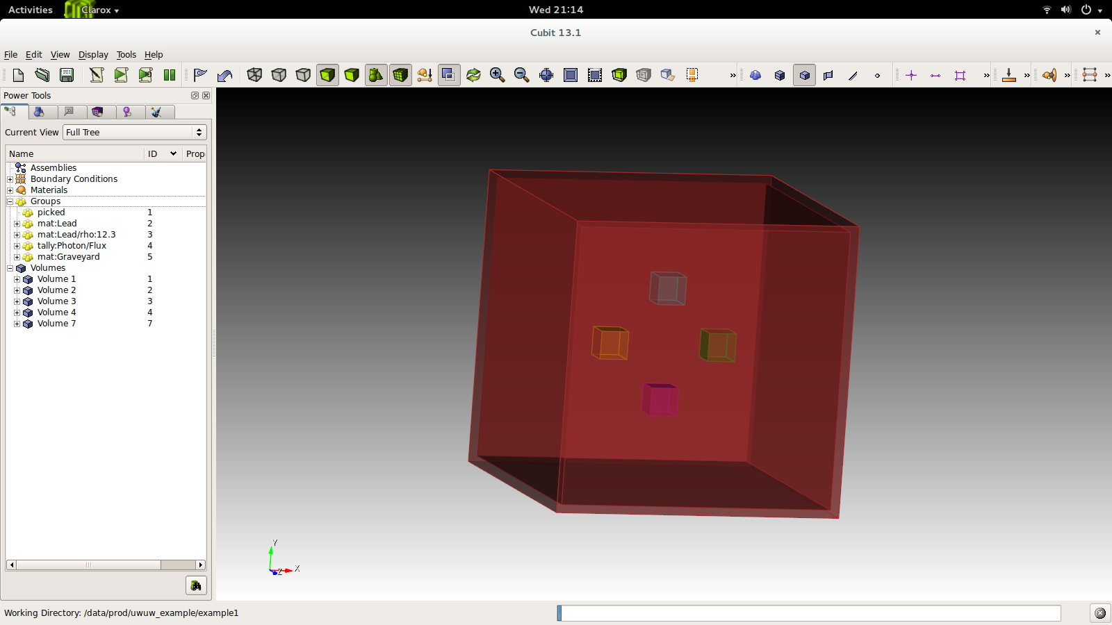
Open Cubit, and let’s place some volumes to create our first problem. We will create 4 cubes of side 10 cm, shifting each in a different direction.

CUBIT> brick x 10
CUBIT> move Volume 1 x 20 include_merged
CUBIT> group "mat:Lead" add volume 1
CUBIT> group "tally:Photon/Flux" add volume 1
CUBIT> brick x 10
CUBIT> move Volume 2 x -20 include_merged
CUBIT> group "mat:Lead" add volume 2
CUBIT> group "tally:Photon/Flux" add volume 2
CUBIT> brick x 10
CUBIT> move Volume 3 y -20 include_merged
CUBIT> group "mat:Lead/rho:12.3" add volume 3
CUBIT> group "tally:Photon/Flux" add volume 3
CUBIT> brick x 10
CUBIT> move Volume 4 y 20 include_merged
CUBIT> group "mat:Lead/rho:12.3" add volume 4
CUBIT> group "tally:Photon/Flux" add volume 4
CUBIT> brick x 100
CUBIT> brick x 105
CUBIT> subtract volume 5 from volume 6
CUBIT> group "mat:Graveyard" add volume 7
CUBIT> imprint body all
CUBIT> merge all
CUBIT> set attribute on
CUBIT> export acis "example.sat" overwrite

You will end up with something like this.

The file is now ready for preprocessing. First we must facet the file:

$ dagmc_preproc example.sat -o example.h5m

Now we can insert all the material data we need:

$ uwuw_preproc example.h5m -l \
      $HOME/.local/lib/python2.7/site-packages/pyne/nuc_data.h5

Your output from this step should look exactly the same as this:

Making new material with name      : mat:Lead
                 with fluka_name:     LEAD
Making new material with name      : mat:Lead/rho:12.3
                 with fluka_name:    LEAD1
Photon PHFL1 3
Photon PHFL2 3
Photon PHFL3 3
Photon PHFL4 3
writing material, mat:Leadwriting material,     LEAD to file example.h5m
writing material, mat:Lead/rho:12.3writing material,    LEAD1 to file example.h5m
Writing tally PHFL1 to file example.h5m
Writing tally PHFL2 to file example.h5m
Writing tally PHFL3 to file example.h5m
Writing tally PHFL4 to file example.h5m

So we see echoed back to us that we requested a graveyard and two different material assignments: one for lead, as defined in the material library, and another kind of lead at a different density than the library version. We also see that 4 tallies were requested: the photon flux in each volume.

Example input¶

We are now ready to run DAGMC, once we have made the input deck for each Monte Carlo code. We wish to simulate 10^5 photons with energy 1 MeV emitted isotropically from the point (0,0,0). The inputs for MCNP5 and FLUKA are shown below.

MCNP5 example: let us call this mcnp.inp.

example of UWUW
c notice no cell cards
c notice no surface cards
c notice no blank lines!
sdef x=0.0 y=0.0 z=0.0 par=2 erg=1.0
c notice no materials
c notice no tallies
mode p
nps 1e5
print

FLUKA example: let us called this fluka.inp.

TITLE
* Set the defaults for precision simulations
DEFAULTS                                                              PRECISIO
* Define the beam characteristics
BEAM          -0.001             10000.0                              PHOTON
* Define the beam position
BEAMPOS           0.        0.        0.
* Notice the FLUGG section
GEOBEGIN                                                              FLUGG
GEOEND
* notice no material assignments
* notice no scoring assignments
* ..+....1....+....2....+....3....+....4....+....5....+....6....+....7...
RANDOMIZ         1.0
* Set the number of primary histories to be simulated in the run
EMF
START           1.E5
STOP

DAG-MCNP5 run¶

Now we are ready to run the first DAG-MCNP5 example.

$ mcnp5 i=mcnp.inp g=example.h5m

You should see something like this on screen.

The implicit complement's total surface area = 128550
This problem is using DAGMC version    1.000 w/ DagMC r   0
Using default writer WriteHDF5 for file fcad
/mnt/data/prod/uwuw_example/web_example/example.h5m
Materials present in the h5m file
mat:Lead
mat:Lead/rho:12.3
Tallies present in the h5m file
PHFLUX1
PHFLUX2
PHFLUX3
PHFLUX4
Going to write an lcad file = lcad
Tallies
          Thread Name & Version = MCNP5, 1.60
          Copyright LANS/LANL/DOE - see output file
                                  _
            ._ _    _  ._   ._   |_
            | | |  (_  | |  |_)   _)
                            |

comment.  photon   importances have been set equal to 1.
comment. using random number generator  1, initial seed = 19073486328125
Turned OFF ray firing on full CAD model.
Set overlap thickness = 0
imcn   is done

 warning.  material        1 has been set to a conductor.
 warning.  material        2 has been set to a conductor.

                           ctm =        0.00   nrn =                 0
dump    1 on file runtpe   nps =           0   coll =                0
  xact   is done

cp0 =   0.01
run terminated when      100000  particle histories were done.

                             ctm =        0.05   nrn =            900033
dump    2 on file runtpe   nps =      100000   coll =            56221
mcrun  is done

Feel free to examine the output of the run, but this is only a simple example of what to expect.

FluDAG run¶

For FluDAG, first we produce the mat.inp snippet file. This must then be pasted into the full FLUKA input deck.

$ mainfludag example.h5m

The mat.inp file should look like

*...+....1....+....2....+....3....+....4....+....5....+....6....+....7...
ASSIGNMA       LEAD1        1.
ASSIGNMA       LEAD1        2.
ASSIGNMA       LEAD2        3.
ASSIGNMA       LEAD2        4.
ASSIGNMA    BLCKHOLE        5.
ASSIGNMA      VACUUM        6.
*...+....1....+....2....+....3....+....4....+....5....+....6....+....7...
MATERIAL         82.   207.217     11.35       26.                    LEAD1
MATERIAL         82.   207.217      12.3       27.                    LEAD2
*...+....1....+....2....+....3....+....4....+....5....+....6....+....7...
* UW**2 tallies
* PHFLUX1
USRTRACK         1.0    PHOTON       -21        1.1.0000e+03     1000.PHFLUX1
USRTRACK       10.E1     1.E-3                                               &
* PHFLUX2
USRTRACK         1.0    PHOTON       -21        2.1.0000e+03     1000.PHFLUX2
USRTRACK       10.E1     1.E-3                                               &
* PHFLUX3
USRTRACK         1.0    PHOTON       -21        3.1.0000e+03     1000.PHFLUX3
USRTRACK       10.E1     1.E-3                                               &
* PHFLUX4
USRTRACK         1.0    PHOTON       -21        4.1.0000e+03     1000.PHFLUX4
USRTRACK       10.E1     1.E-3                                               &

At this point you will need to add two lines to the input file manually. This is because the component of the code which identifies neutron cross section data is not yet complete.

*...+....1....+....2....+....3....+....4....+....5....+....6....+....7....+....
LOW-MAT        LEAD1       82.       -2.      296.                    LEAD
LOW-MAT        LEAD2       82.       -2.      296.                    LEAD

The lines above must be pasted into the FLUKA input and then run as you would a native FLUKA problem, with the exception that we give the rfluka script an executable argument and a new -d argument, which specifies the geometry filename.

$ $FLUPRO/flutil/rfluka -N0 -M1 -e mainfludag -d example.h5m fluka.inp

The code should run and successfully produce screen output similar to the following. (The filepaths will change according to your system, as will the numerical part of “fluka_26362”.)

$TARGET_MACHINE = Linux
$FLUPRO = /mnt/data/opt/fluka/fluka/

Initial seed already existing
Running fluka in /mnt/data/prod/uwuw_example/web_example/fluka_26362

======================= Running FLUKA for cycle # 1 =======================

Removing links
Removing temporary files
Saving output and random number seed
Saving additional files generated
Moving fort.21 to /mnt/data/prod/uwuw_example/web_example/fluka001_fort.21
End of FLUKA run

Dag-Geant4 run¶

Dag-Geant4 is probably the most trivial of all the UW²-enabled codes to run. Copy the vis.mac file from DAGMC/geant4/app/vis.mac.

$ DagGeant4 example.h5m

After some loading you should see a GUI window open (if you built Geant4 with visualization enabled). You can then use the Geant4 general particle source to emulate the behaviour of the previous two codes.

Idle> /gps/particle gamma
Idle> /gps/ang/type iso
Idle> /gps/energy 1.0 MeV

Now we are ready to run.

Idle> /run/beamOn 1000000